Appearance
Vector Operations
This lesson explores fundamental vector operations in linear algebra, their crucial role in quantitative trading and machine learning, and their practical implementation using Python.
Introduction
Hey there! Welcome back! We're diving straight into the action with vector operations. You already know what vectors are, so we'll jump directly into how we manipulate them. This lesson focuses on the essential operations: addition, subtraction, scalar multiplication, dot product, cross product, and the scalar component. These aren't just abstract mathematical concepts; they are the workhorses of quantitative trading and machine learning. We'll explore these operations in detail, including the rules that govern them, and then see their practical applications in finance, implemented in Python. Get ready to solidify your understanding and see how these operations power sophisticated trading strategies and models.
Operations
Addition
Definition: Vector addition combines two vectors element-wise, resulting in a new vector.
Formula:
Rules and Properties:
- Commutativity:
(The order of addition doesn't matter.) - Associativity:
(You can group the additions in any order.) - Identity Element: There exists a zero vector,
, such that for any vector . - Inverse Element: For every vector
, there exists an additive inverse, , such that .
Geometric Interpretation: Vector addition can be visualized using the parallelogram rule. Place the tail of vector b at the head of vector a. The resulting vector, a + b, is the diagonal of the parallelogram formed by a and b, starting from the tail of a.
python
import matplotlib.pyplot as plt
import numpy as np

a = np.array([2, 1])
b = np.array([1, 3])

plt.figure(figsize=(5, 5))
plt.quiver(0, 0, a[0], a[1], angles='xy', scale_units='xy', scale=1, color='r', label='a')
plt.quiver(0, 0, b[0], b[1], angles='xy', scale_units='xy', scale=1, color='b', label='b')
plt.quiver(a[0], a[1], b[0], b[1], angles='xy', scale_units='xy', scale=1, color='b', linestyle='dashed') # Show how b starts at the head of a
plt.quiver(0, 0, (a + b)[0], (a + b)[1], angles='xy', scale_units='xy', scale=1, color='g', label='a+b')

plt.xlim(-1, 5)
plt.ylim(-1, 5)
plt.axhline(0, color='black',linewidth=0.5)
plt.axvline(0, color='black',linewidth=0.5)
plt.grid(True)
plt.legend()
plt.title("Vector Addition")
plt.show()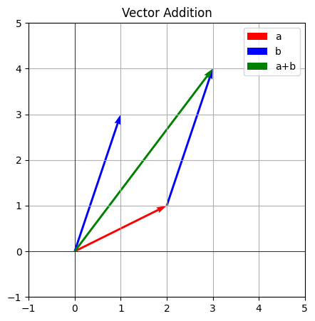
Connection to Advanced Topics: Vector addition is fundamental to defining vector spaces.
Subtraction
Definition: Vector subtraction finds the difference between two vectors element-wise.
Formula:
Rules and Properties:
- Not Commutative:
(The order does matter.) - Relationship to Addition:
(Subtraction is equivalent to adding the negative of the second vector.)
Geometric Interpretation: Place the tails of a and b at the same point. The vector a - b points from the head of b to the head of a. Alternatively, you can visualize it as adding a to the negative of b (-b).
python
import matplotlib.pyplot as plt
import numpy as np

a = np.array([2, 1])
b = np.array([1, 3])

plt.figure(figsize=(5, 5))
plt.quiver(0, 0, a[0], a[1], angles='xy', scale_units='xy', scale=1, color='r', label='a')
plt.quiver(0, 0, b[0], b[1], angles='xy', scale_units='xy', scale=1, color='b', label='b')
plt.quiver(0, 0, (a - b)[0], (a - b)[1], angles='xy', scale_units='xy', scale=1, color='purple', label='a-b')
plt.quiver(0, 0, (b - a)[0], (b - a)[1], angles='xy', scale_units='xy', scale=1, color='orange', label='b-a')

plt.xlim(-3, 4)
plt.ylim(-3, 4)
plt.axhline(0, color='black',linewidth=0.5)
plt.axvline(0, color='black',linewidth=0.5)
plt.grid(True)
plt.legend()
plt.title("Vector Subtraction")
plt.show()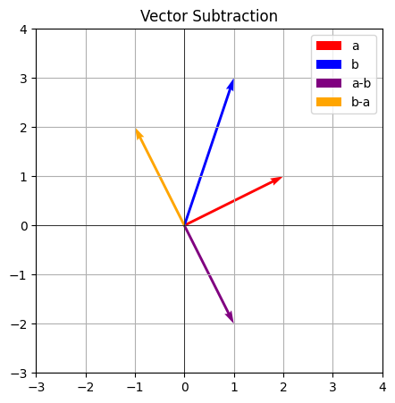
Connection to Advanced Topics: Vector subtraction is used in calculating distances between vectors.
Scalar Multiplication
Definition: Scalar multiplication multiplies a vector by a scalar (a single number). Formula:
Rules and Properties:
- Associativity:
(where c and d are scalars) - Distributivity over Vector Addition:
- Distributivity over Scalar Addition:
- Identity Element:
- Zero Element:
Geometric Interpretation: Scalar multiplication scales the magnitude (length) of the vector.
python
import matplotlib.pyplot as plt
import numpy as np

a = np.array([1, 2])
c1 = 2
c2 = 0.5
c3 = -1

plt.figure(figsize=(6, 6))
plt.quiver(0, 0, a[0], a[1], angles='xy', scale_units='xy', scale=1, color='r', label='a')
plt.quiver(0, 0, c1*a[0], c1*a[1], angles='xy', scale_units='xy', scale=1, color='g', label='2a')
plt.quiver(0, 0, c2*a[0], c2*a[1], angles='xy', scale_units='xy', scale=1, color='b', label='0.5a')
plt.quiver(0, 0, c3*a[0], c3*a[1], angles='xy', scale_units='xy', scale=1, color='purple', label='-1a')

plt.xlim(-3, 4)
plt.ylim(-3, 4)
plt.axhline(0, color='black',linewidth=0.5)
plt.axvline(0, color='black',linewidth=0.5)
plt.grid(True)
plt.legend()
plt.title("Scalar Multiplication")
plt.show()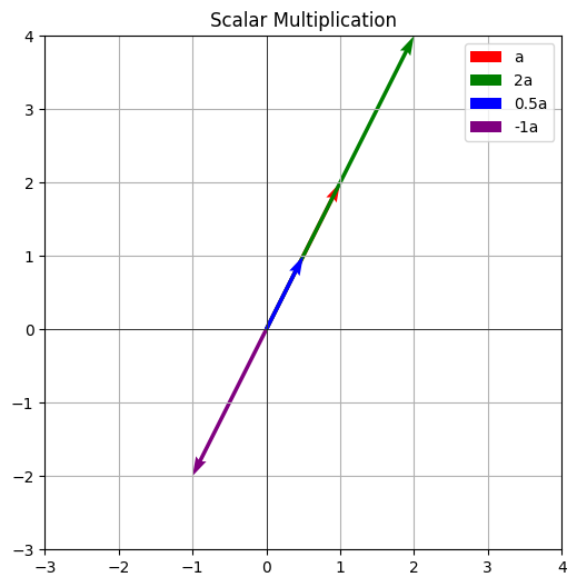
Connection to Advanced Topics: Scalar multiplication, along with vector addition, defines the concept of a linear combination.
Dot Product
Definition: The dot product (or scalar product) of two vectors is a scalar value.
Formula:
Rules and Properties:
- Commutativity:
- Distributivity:
- Scalar Multiplication:
- Orthogonality:
if and only if and are orthogonal. - Relationship to Magnitude and Angle:
Geometric Interpretation: The dot product is related to the projection of one vector onto another.
Python
import matplotlib.pyplot as plt
import numpy as np

a = np.array([3, 1])
b = np.array([1, 2])

# Calculate the projection of a onto b
proj_a_on_b = (np.dot(a, b) / np.dot(b, b)) * b

plt.figure(figsize=(6, 6))
plt.quiver(0, 0, a[0], a[1], angles='xy', scale_units='xy', scale=1, color='r', label='a')
plt.quiver(0, 0, b[0], b[1], angles='xy', scale_units='xy', scale=1, color='b', label='b')
plt.quiver(0, 0, proj_a_on_b[0], proj_a_on_b[1], angles='xy', scale_units='xy', scale=1, color='g', label='proj_a_on_b')

plt.xlim(-1, 4)
plt.ylim(-1, 4)
plt.axhline(0, color='black',linewidth=0.5)
plt.axvline(0, color='black',linewidth=0.5)
plt.grid(True)
plt.legend()
plt.title("Dot Product and Projection")
plt.show()
Connection to Advanced Topics: The dot product is used extensively in calculating angles, defining orthogonality, and calculating projections.
Cross Product
Definition: The cross product of two 3-dimensional vectors is a new vector perpendicular to both.
Formula:
Rules and Properties:
- Anti-Commutativity:
- Distributivity:
- Scalar Multiplication:
- Parallel Vectors:
if and only if and are parallel. - Magnitude and Angle:
- Right-Hand Rule: Determines the direction of
.
Geometric Interpretation: The cross product results in a vector perpendicular to the plane defined by the input vectors. Its magnitude represents the area of the parallelogram.
Python
import matplotlib.pyplot as plt
import numpy as np
from mpl_toolkits.mplot3d import Axes3D

a = np.array([1, 2, 0])
b = np.array([0, 1, 2])
cross_product = np.cross(a, b)

fig = plt.figure(figsize=(7, 7))
ax = fig.add_subplot(111, projection='3d')

ax.quiver(0, 0, 0, a[0], a[1], a[2], color='r', label='a')
ax.quiver(0, 0, 0, b[0], b[1], b[2], color='b', label='b')
ax.quiver(0, 0, 0, cross_product[0], cross_product[1], cross_product[2], color='g', label='a x b')

ax.set_xlim([0, 4])
ax.set_ylim([0, 4])
ax.set_zlim([0, 4])
ax.set_xlabel('X')
ax.set_ylabel('Y')
ax.set_zlabel('Z')
ax.legend()
ax.set_title("Cross Product")
plt.show()
Connection to Advanced Topics: Used in computer graphics, physics, and geometric calculations.
Scalar Component
Definition: The scalar component of vector a onto vector b tells the magnitude of the projection of a onto b.
Formula: comp (a onto b) = (|a| cos θ) = (a · b) / |b|
Rules and Properties:
- Relationship to Dot Product: Derived from the dot product.
- Sign: Indicates the direction of the projection.
- If b is a unit vector, the formula simply becomes a · b
Geometric Interpretation: The length of the shadow of vector a cast onto vector b. The code for visualizing this is the same as for the dot product's projection. Refer to the Dot Product's geometric interpretation code.
Connection to Advanced Topics: Used to calculate the vector projection and in orthogonal decomposition.
Application to Quantitative Trading and ML
Portfolio Optimization (Mean-Variance Optimization)
We represent portfolio weights as a vector w. Expected returns of assets are another vector
Risk Management (Value at Risk - VaR)
VaR calculations often involve vectors of asset returns and weights. Calculating portfolio standard deviation, a key component of VaR, uses the same vector operations as portfolio optimization. Understanding the properties of vector subtraction and the dot product is essential for interpreting VaR results.
Trading Signal Generation
Technical indicators, like moving averages, are calculated using vector operations. A simple moving average is a dot product between prices and uniform weights. Differences between moving averages (MACD) involve vector subtraction. The distributive property of the dot product over vector addition is crucial for efficiently calculating these indicators.
Machine Learning Feature Engineering
Creating new features often involves vector operations. The difference (vector subtraction) between two features or scaling a feature (scalar multiplication) are common examples. The rules of these operations ensure that the new features are mathematically sound.
Machine Learning Model Training
Many machine learning algorithms (linear regression, SVMs, neural networks) rely heavily on vector operations. Weighted sums of inputs are dot products. Understanding the properties of the dot product is vital for understanding how these models work and for debugging them. For instance, if the dot product between input features and weights is consistently very large or very small, it might indicate issues with feature scaling.
Market Microstructure Analysis
Analyzing order book data often involves calculating vector distances, which can reveal information about the similarity of liquidity profiles, and calculating angles between vectors for comparing order flow directions.
Python Implementation
Python
import numpy as np
import matplotlib.pyplot as plt
from mpl_toolkits.mplot3d import Axes3D

# --- Vector Operations ---
a = np.array([1, 2, 3])
b = np.array([4, 5, 6])
c = 2

# Addition
print("Addition:", a + b)  # Demonstrates element-wise addition

# Subtraction
print("Subtraction:", a - b) # Demonstrates element-wise subtraction

# Scalar Multiplication
print("Scalar Multiplication:", c * a) # Demonstrates scalar multiplication

# Dot Product
print("Dot Product:", np.dot(a, b))  # Or a @ b. Demonstrates dot product calculation

# Cross Product (only for 3D vectors)
print("Cross Product:", np.cross(a, b))  # Demonstrates cross product

# Scalar Component of a onto b
dot_product = np.dot(a,b)
magnitude_b = np.linalg.norm(b)
scalar_component = dot_product / magnitude_b
print("Scalar Component of a onto b:", scalar_component)

# --- Portfolio Optimization Example (Simplified) ---
# Assume we have two assets with expected returns and covariance matrix:
mu = np.array([0.10, 0.15])  # Expected returns of 10% and 15%
covariance_matrix = np.array([[0.01, 0.005],
                             [0.005, 0.0225]])

# Let's calculate the portfolio return and variance for a specific portfolio:
weights = np.array([0.6, 0.4])  # 60% in asset 1, 40% in asset 2

portfolio_return = np.dot(weights, mu) # Dot product for portfolio return
portfolio_variance = np.dot(weights.T, np.dot(covariance_matrix, weights)) # Matrix-vector multiplication (uses dot product)
portfolio_std_dev = np.sqrt(portfolio_variance) # Square root for standard deviation

print(f"Portfolio Return: {portfolio_return:.4f}")
print(f"Portfolio Standard Deviation: {portfolio_std_dev:.4f}")

# --- Visualization (2D Vectors) ---
# Visualize vector addition and subtraction
a_2d = np.array([2, 1])
b_2d = np.array([1, 3])

plt.figure(figsize=(6, 6))
plt.quiver(0, 0, a_2d[0], a_2d[1], angles='xy', scale_units='xy', scale=1, color='r', label='a')
plt.quiver(0, 0, b_2d[0], b_2d[1], angles='xy', scale_units='xy', scale=1, color='b', label='b')
plt.quiver(a_2d[0], a_2d[1], b_2d[0], b_2d[1], angles='xy', scale_units='xy', scale=1, color='b', linestyle='dashed') # Show how b starts at the head of a
plt.quiver(0, 0, (a_2d + b_2d)[0], (a_2d + b_2d)[1], angles='xy', scale_units='xy', scale=1, color='g', label='a+b')
plt.quiver(0, 0, (a_2d - b_2d)[0], (a_2d - b_2d)[1], angles='xy', scale_units='xy', scale=1, color='purple', label='a-b')

plt.xlim(-2, 5)
plt.ylim(-1, 5)
plt.axhline(0, color='black',linewidth=0.5)
plt.axvline(0, color='black',linewidth=0.5)
plt.grid(True)
plt.legend()
plt.title("Vector Addition and Subtraction")
plt.show()

# --- Visualization (3D Vectors & Cross Product) ---
a_3d = np.array([1, 2, 3])
b_3d = np.array([4, 1, 2])
cross_product = np.cross(a_3d, b_3d)

fig = plt.figure(figsize=(8, 8))
ax = fig.add_subplot(111, projection='3d')

# Plot vectors
ax.quiver(0, 0, 0, a_3d[0], a_3d[1], a_3d
Exercises/Problems
Exercise 1: Basic Operations
md
Problem Statement:

Given vectors u = [4, -1, 2] and v = [1, 3, -2], calculate:

a) u + v
b) u - v
c) 2u
d) u · v
e) u × v
f) the scalar component of u onto v.

Hints: Use the formulas and NumPy functions.
python
Python
import numpy as np

u = np.array([4, -1, 2])
v = np.array([1, 3, -2])

# a) u + v

print("u + v:", u + v) # Output: [ 5 2 0]

# b) u - v

print("u - v:", u - v) # Output: [ 3 -4 4]

# c) 2u

print("2u:", 2 \* u) # Output: [ 8 -2 4]

# d) u . v

print("u . v:", np.dot(u, v)) # Output: -3

# e) u x v

print("u x v:", np.cross(u, v)) # Output: [-4 10 13]

# f) Scalar component of u onto v

dot_product = np.dot(u, v)
magnitude_v = np.linalg.norm(v)
scalar_comp = dot_product / magnitude_v
print("Scalar Component of u onto v: ", scalar_comp) # Output: -0.7905694150420949
Exercise 2: Portfolio Optimization
md
You have two assets with weights w = [0.7, 0.3]
Expected returns are μ = [0.12, 0.08]
The covariance matrix is:
[[0.02, 0.008],
 [0.008, 0.01]]

Calculate the portfolio return and standard deviation.

Hints: Use the dot product for return and matrix-vector
multiplication for variance.
python
import numpy as np

w = np.array([0.7, 0.3])
mu = np.array([0.12, 0.08])
covariance_matrix = np.array([[0.02, 0.008],[0.008, 0.01]])

portfolio_return = np.dot(w, mu)
portfolio_variance = np.dot(w.T, np.dot(covariance_matrix, w))
portfolio_std_dev = np.sqrt(portfolio_variance)

print(f"Portfolio Return: {portfolio_return:.4f}")
# Output: 0.1080

print(f"Portfolio Standard Deviation: {portfolio_std_dev:.4f}")
# Output: 0.1296
md
The portfolio return is calculated as the dot product
of the weights and expected returns. The portfolio
variance uses the formula wᵀΣw, implemented with nested
dot products. The standard deviation is the square root
of the variance.
Exercise 3: Orthogonal and Parallel Vectors
md
Determine if the following pairs of vectors are orthogonal,
parallel, or neither:

a) [2, -4] and [-1, -0.5]
b) [1, 2, 3] and [4, 5, -6]
c) [1, 0, 0] and [0, 0, 1]

Hints: For orthogonality, check if the dot product is zero.
For parallel vectors (in 3D), check if the cross product is
the zero vector. For 2D vectors, you can check if one is a
scalar multiple of the other.
python
import numpy as np

# a)
a1 = np.array([2, -4])
a2 = np.array([-1, -0.5])
print("a) Dot product:", np.dot(a1, a2))
# Output: 0. Orthogonal.


# b)
b1 = np.array([1, 2, 3])
b2 = np.array([4, 5, -6])
print("b) Dot product:", np.dot(b1, b2))
# Output: -4. Neither.
print("b) Cross product:", np.cross(b1, b2))
# Output: [-27 18 -3]. Neither.


# c)
c1 = np.array([1, 0, 0])
c2 = np.array([0, 0, 1])
print("c) Dot product:", np.dot(c1, c2))
# Output: 0. Orthogonal.
md
a) The dot product is 0, so the vectors are orthogonal.

b) The dot product is not 0, so they are not orthogonal.
The cross product is not the zero vector, so they are
not parallel. Therefore, they are neither.

c) The dot product is 0, so the vectors are orthogonal.
Dive Deeper
Linear Algebra Textbooks
- "Introduction to Linear Algebra" by Gilbert Strang: A classic, comprehensive textbook.
- "Linear Algebra and Its Applications" by David C. Lay: Another excellent textbook with a focus on applications.
- "Linear Algebra Done Right" by Sheldon Axler: A more abstract, proof-based approach.
Quantitative Finance Books
- "Options, Futures, and Other Derivatives" by John C. Hull: A standard reference for derivatives pricing, which uses linear algebra extensively.
- "Quantitative Trading: How to Build Your Own Algorithmic Trading Business" by Ernest P. Chan: A practical guide to building trading strategies, with many examples using vector operations.
- "Advances in Financial Machine Learning" by Marcos Lopez de Prado: Covers more advanced topics, including how linear algebra concepts underpin many machine learning techniques used in finance.
Online Resources
- MIT OpenCourseware (18.06 Linear Algebra): Gilbert Strang's famous linear algebra course, available online for free. Includes video lectures, problem sets, and solutions.
- Khan Academy (Linear Algebra): A great resource for learning the basics of linear algebra, with clear explanations and interactive exercises.
- 3Blue1Brown (Essence of Linear Algebra): A YouTube series with fantastic visualizations that provide intuitive understanding of linear algebra concepts.
Advanced Topics
- Eigenvalues and Eigenvectors: These are crucial for understanding the behavior of linear transformations and are used in many areas of quantitative finance, such as Principal Component Analysis (PCA) for dimensionality reduction and risk management.
- Matrix Decompositions (SVD, QR, Cholesky): These decompositions are used to solve linear systems, perform least squares regression, and are fundamental to many numerical algorithms.
- Vector Spaces and Subspaces: A more abstract understanding of vector spaces is essential for advanced work in linear algebra and functional analysis.
- Linear Transformations: Understanding how matrices represent linear transformations provides a deeper understanding of how many financial models work.
- Norms and Metrics: Different ways of measuring the "size" or "distance" between vectors, with applications in optimization and machine learning (e.g., regularization).